Master Water Modeling &
Constructed Wetland Design
A complete interactive course to understand the science, design principles, and real-world application of AquaSai's Multi-Stage Recirculating (MSR) constructed wetland systems.
What You'll Master
This course takes you from first principles to professional practice. You will understand why constructed wetlands work at a molecular and ecosystem level, how to design them using verified scientific models, and where AquaSai has applied them in the real world.
The AquaSai Ecosystem
AquaSai is a nature-based water treatment venture anchored in the MSR (Multi-Stage Recirculating) Constructed Wetland — a modular, solar-powered, IoT-monitored system that achieves advanced wastewater treatment using engineered plant communities, stratified substrate, and controlled hydraulics.
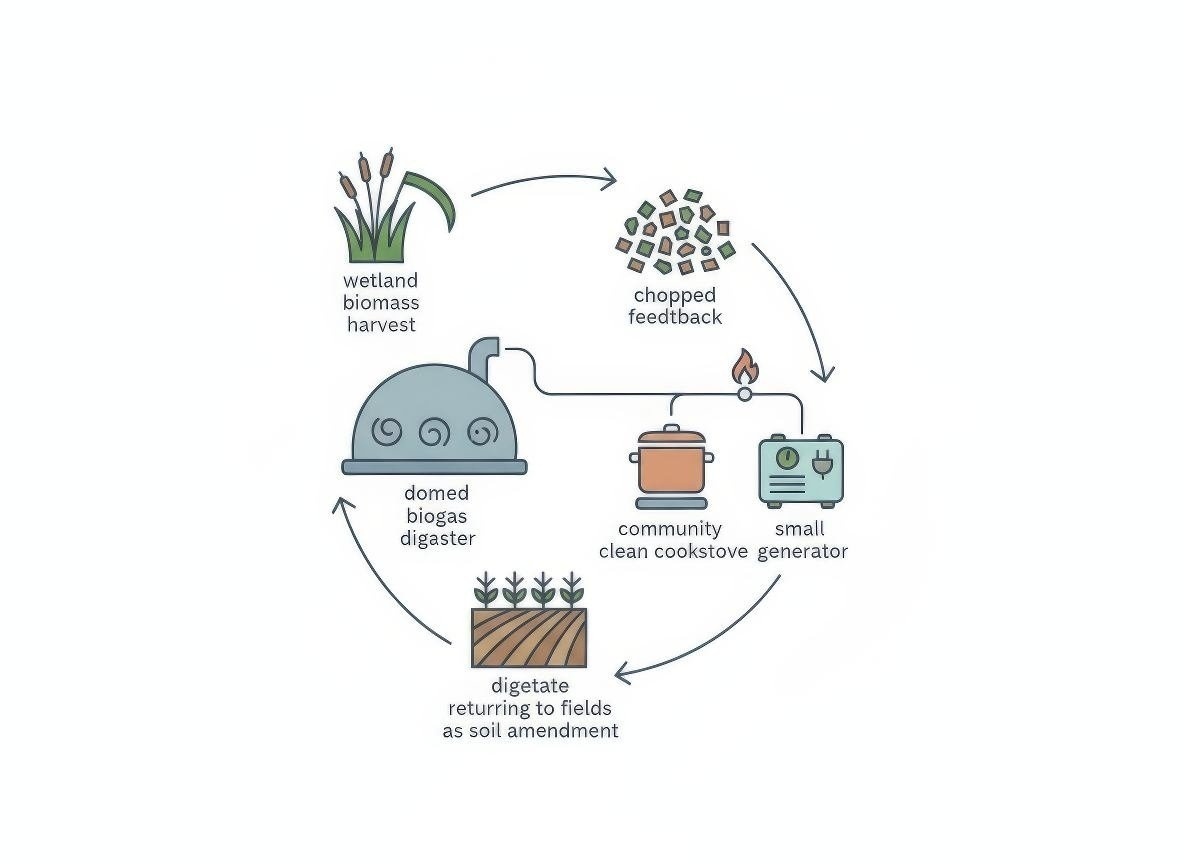
Unlike conventional treatment plants that consume energy and chemicals, AquaSai systems generate ecosystem services: they sequester carbon, support biodiversity, produce biomass for biogas, and integrate into the local Water–Energy–Food nexus.
Science-First
Every design parameter is derived from peer-reviewed models: Kadlec & Wallace 2009, HYDRUS-CW2D, CWM1, Arrhenius kinetics.
Off-Grid Ready
Solar-powered pumping, IoT monitoring, minimal OPEX. Designed for remote and peri-urban communities.
Globally Deployed
Koh Phangan (Thailand), Kathmandu Bagmati (Nepal), ETBAR Tenerife (Spain). Each adapts MSR to local ecology.
Verified Performance
Pre-validated with HYDRUS-CW2D simulations. Target BOD ≤ 10 mg/L, TSS ≤ 10 mg/L, E.coli ≤ 1000 CFU/100mL.
An AquaSai MSR constructed wetland can achieve BOD ≤ 10 mg/L and E.coli ≤ 1,000 CFU/100 mL using only plants, sunlight, gravity and gravel — with zero chemical dosing and a fraction of the energy of a conventional activated-sludge plant.
This course distils methods proven across three live AquaSai deployments — the Koh Phangan resort wetland (Thailand), the Bagmati river-edge system (Kathmandu, Nepal) and the ETBAR Ensenada Pelada coastal pilot (Tenerife, Spain).
— AquaSai engineering team🌐 AquaSai MSR Ecosystem — Interactive Knowledge Map
Hover over any node to explore. Click to reveal details about each system component.
- Distinguish between FWS, HSSF, VSSF and MSR constructed wetland typologies
- Explain the six treatment mechanisms operating simultaneously in AquaSai MSR
- Describe how recirculation links nitrification and denitrification across stages
- Define primary, secondary and tertiary treatment roles in a multi-stage system
What is a Constructed Wetland?
A Constructed Wetland (CW) is an engineered shallow basin planted with aquatic macrophytes, filled with porous substrate (gravel, sand, coconut coir), through which wastewater flows and is treated by physical, chemical, and biological mechanisms working simultaneously.
Unlike a natural wetland that is preserved for biodiversity, a CW is deliberately designed and sized to achieve specific treatment targets — BOD removal, nitrification, denitrification, phosphorus sorption — validated against mathematical models.
Types of Constructed Wetlands
🌊 FWS — Free Water Surface
Water flows above substrate, exposed to atmosphere. Excellent for tertiary polishing, wildlife habitat. Lower capital, moderate BOD removal.
🔄 HSSF — Horizontal Subsurface Flow
Water flows horizontally through gravel below surface. Anaerobic/anoxic zones → excellent denitrification. Most common CW type worldwide.
⬇️ VSSF — Vertical Subsurface Flow
Water loaded from top, percolates down. Intermittent dosing creates aerobic conditions → excellent nitrification. Energy-efficient via gravity.
🔀 MSR — Multi-Stage Recirculating
AquaSai's integrated design: combines HSSF + VSSF + FWS + recirculation loop in sequence. Achieves what no single type can match alone.
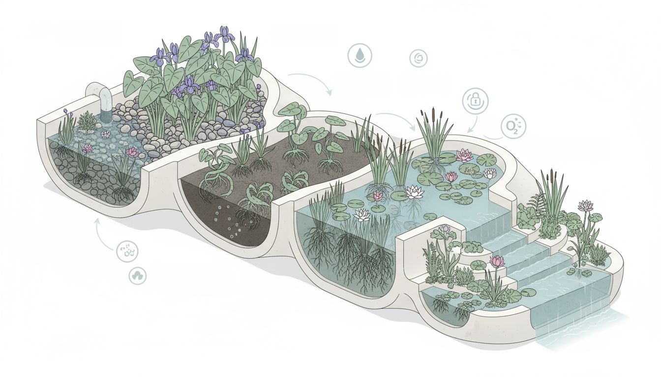
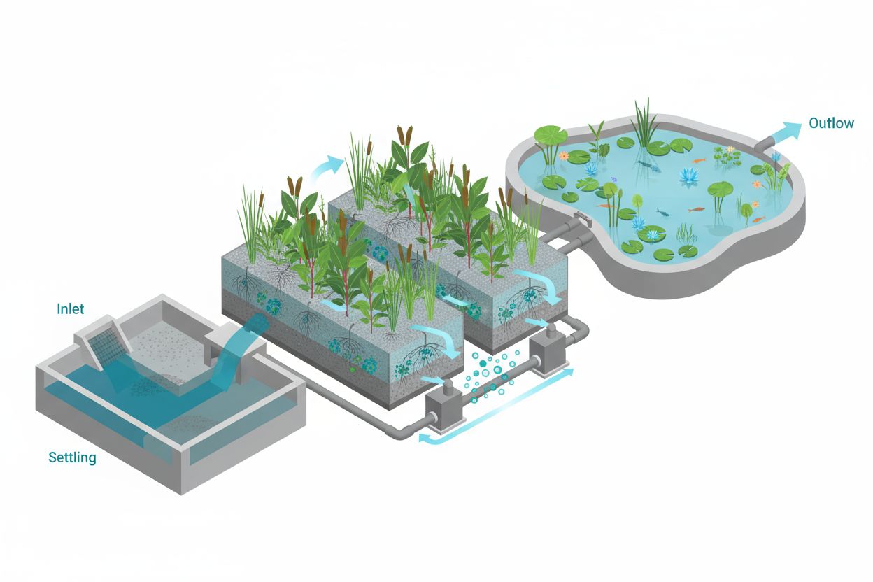
The AquaSai MSR — 4-Stage Treatment Train
The MSR is the heart of every AquaSai project. Flow the wastewater through all four stages by clicking each box:
Why MSR Out-Performs Single-Stage Systems
Each treatment mechanism has conditions under which it thrives — anaerobic bacteria need zero oxygen, nitrifiers need high oxygen, denitrifiers need anoxic conditions with available carbon. A single bed cannot simultaneously optimize all of them.
The MSR resolves this by staging: each cell operates in its optimal redox window, and the recirculation loop allows partially nitrified effluent to re-enter the HSSF, providing the nitrate that denitrifiers need and the carbon that nitrifiers lack.

🗺️ Constructed Wetland Type Comparison — Knowledge Map
Hover each node to see hydraulic and treatment characteristics. All four types combine in the AquaSai MSR.
📝 Module 1 Quiz
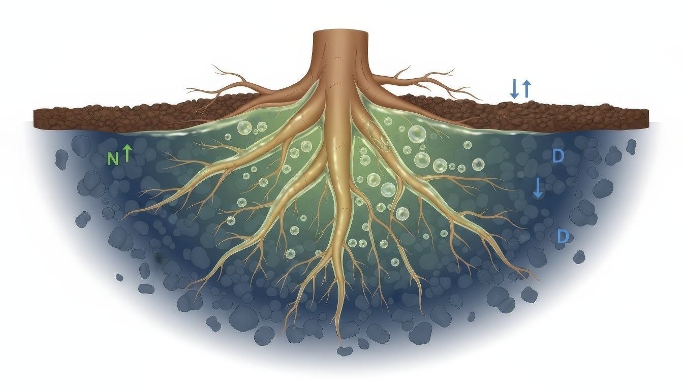
A single reed (Phragmites australis) can transport oxygen down to its roots and leak it into the substrate — creating aerobic micro-zones millimetres from anoxic ones. This radial oxygen loss is why one AquaSai MSR bed can host nitrifiers and denitrifiers side by side.
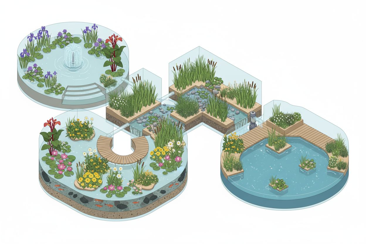
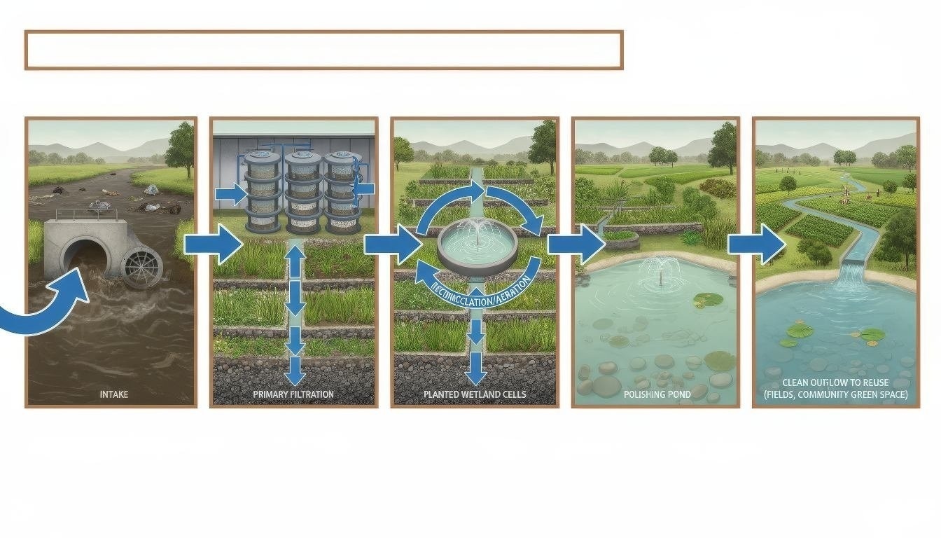
Every AquaSai MSR sequences HSSF → VSSF → FWS with a recirculation loop, so each cell operates in its optimal redox window instead of compromising in a single bed. The cutaway renders above are drawn from real AquaSai project schematics.
— AquaSai MSR design library- MSR is a multi-stage reed bed system combining HSSF, VSSF, FWS and recirculation
- VSSF cells create the aerobic conditions needed for nitrification
- The recirculation loop enables denitrification by returning nitrate-rich effluent to the anoxic HSSF stage
- Stage 1 pre-treatment (primary settlement) removes 40–55% BOD before the wetland beds
- Apply Darcy's Law (Q = K·i·A) to calculate flow velocity through porous substrate
- Compute HLR and HRT for any given system geometry and flow
- Predict how porosity, bed depth and surface area affect hydraulic retention time
- Identify causes and remediation strategies for short-circuiting and clogging
Darcy's Law — The Foundation of Porous Flow
All subsurface flow in constructed wetlands is governed by Darcy's Law, which relates the volumetric flow rate through a porous medium to the hydraulic gradient and medium properties:
AquaSai gravel: K ≈ 10,000–100,000 m/d (new bed); drops to 500–2,000 m/d after biofilm development.
For HSSF wetlands, the hydraulic conductivity K of the gravel substrate typically ranges from 10,000–100,000 m/d. However, biological clogging (biofilm growth) progressively reduces K over time — a key long-term design consideration that MSR addresses through VSSF pulse dosing that aerates and prevents clogging.
Hydraulic Loading Rate (HLR)
HLR [m³/m²·d = m/d], Q = daily flow [m³/d], As = surface area [m²]
HLR is the most important hydraulic design parameter. It determines contact time, velocity through substrate, and is the core input for the P-k-C* treatment model. Typical AquaSai MSR HLR: 0.05–0.15 m/d (conservative, ensuring full treatment).
Hydraulic Retention Time (HRT)
HRT [days], d = depth [m], n = porosity [–], Q = flow [m³/d]
Porosity (n) of the substrate is the fraction of void space available for water storage. Typical values: gravel n=0.35–0.40, coconut coir n=0.50–0.65. A higher porosity means more water is in contact with biofilm-covered surfaces for longer — better treatment at the same area.
🔢 Interactive Hydraulics Calculator
Key Design Ranges (AquaSai Standard)
| Parameter | HSSF Cell | VSSF Cell | Polishing Pond |
|---|---|---|---|
| HLR (m/d) | 0.05–0.15 | 0.08–0.25 | 0.10–0.30 |
| HRT (days) | 2–5 | 1–3 | 3–7 |
| Depth (m) | 0.4–0.8 | 0.5–0.8 | 0.5–1.5 |
| Porosity | 0.35–0.42 | 0.38–0.45 | N/A (open water) |
| L:W ratio | 3:1 – 10:1 | 1:1 – 2:1 | 1:1 – 3:1 |


📝 Module 2 Quiz
Darcy's Law (1856) — written for sand filters in Dijon — still governs how water creeps through the gravel of a modern constructed wetland. AquaSai sizes every HSSF bed so the hydraulic gradient never exceeds the substrate's conductivity, preventing surface breakout and short-circuiting.
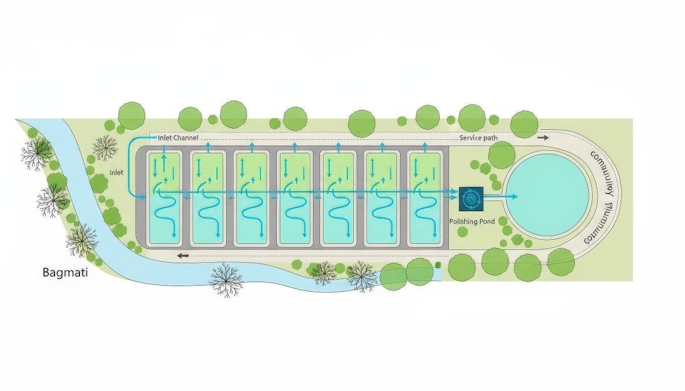
On the Bagmati river-edge system, seasonal monsoon flows swing by an order of magnitude. AquaSai uses HRT and hydraulic-loading design margins (2–5 d in HSSF, 1–3 d in VSSF) so treatment holds in both wet and dry seasons.
— AquaSai Kathmandu project data- Darcy's Law (Q = K·i·A) governs subsurface flow; K is the single most critical substrate parameter
- HLR (m/yr) = Q / As — the primary sizing metric linking flow to treatment area
- HRT (d) = As · d · n / Q — residence time determines treatment contact time
- Biological clogging reduces effective K over time; conservative design uses 20–50% of clean-gravel K
- Apply the P-k-C* model to predict effluent quality from any inlet concentration and area
- Use the Arrhenius equation to temperature-correct rate constants for your site climate
- Explain the role of the irreducible background concentration C* in treatment limits
- Interpret Monod kinetics and half-saturation constants for nitrification biofilms
The P-k-C* Model (Kadlec & Wallace 2009)
The most widely validated model for constructed wetland performance is the P-k-C* (P-order rate constant background concentration) model. For first-order kinetics (P=1), the effluent concentration is:
$k_T$ = Arrhenius-corrected rate constant [m/yr] | HLR = hydraulic loading rate [m/yr]
The C* background concentration represents the irreducible minimum — wetlands cannot achieve zero output because internal biological processes continuously regenerate small amounts of each pollutant. Key C* values: BOD 3.5 mg/L, NH₄-N 0 mg/L, TN 1.5 mg/L, TP 0.02 mg/L.
Arrhenius Temperature Correction
Nitrification (NH₄-N) most temperature-sensitive: θ=1.060 — performance drops ~40% at 10°C vs 20°C.
Rate Constants for Key Pollutants
| Pollutant | k₂₀ (m/yr) | θ (–) | C* (mg/L) | Dominant mechanism |
|---|---|---|---|---|
| BOD | 37.5 | 1.000 | 3.5 | Aerobic/anaerobic degradation |
| NH₄-N | 20.0 | 1.060 | 0.0 | Nitrification (aerobic) |
| NO₃-N | 30.0 | 1.090 | 0.0 | Denitrification (anoxic) |
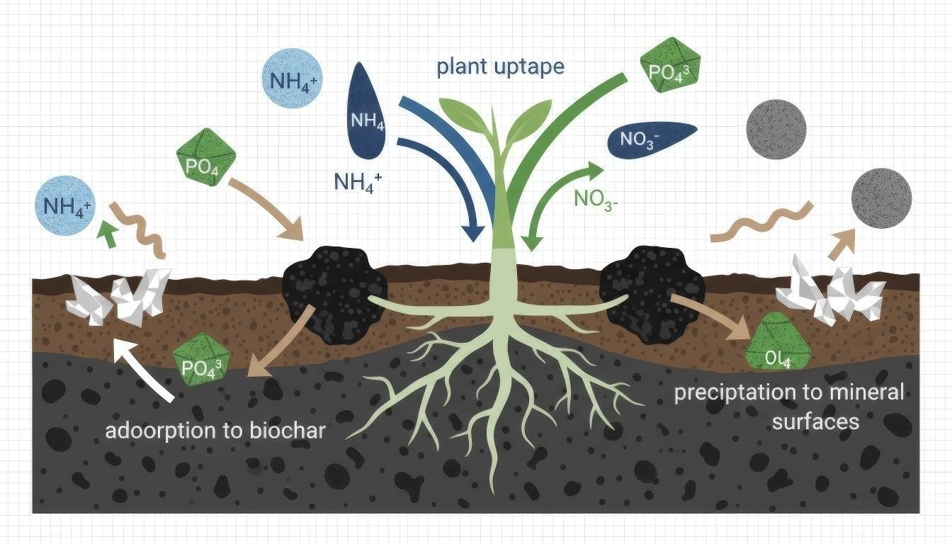
| PO₄-P | 11.0 | 1.010 | 0.02 | Sorption, precipitation |
| TSS | 50.0 | 1.000 | 2.0 | Sedimentation, filtration |
| E.coli | kd=1.5/d | 1.050 | 0.0 | UV, dessication, predation |
⚗️ Live P-k-C* Treatment Calculator
Monod Kinetics — Microbial Growth Rates
Within the biofilm on substrate grains, microbial reaction rates follow Monod kinetics — a saturation function where growth rate approaches a maximum as substrate (food) becomes abundant:
When $S \gg K_s$: zero-order kinetics. When $S \ll K_s$: first-order — this is why P-k-C* works at low effluent concentrations.
When substrate is abundant (S >> Ks), bacteria grow at their maximum rate — zero-order kinetics. When substrate is scarce (S << Ks), growth is proportional to substrate — first-order kinetics. This is why the P-k-C* model (first-order) works so well at low concentrations typical of polishing stages.



🧬 Biochemical Process Web — Pollutant Transformation Pathways
Interactive map of the seven major transformation processes in a constructed wetland. Hover each node for the governing equation and key organisms.
📝 Module 3 Quiz
The rhizosphere — the thin film around plant roots — can hold 10⁸–10⁹ bacteria per gram of substrate. This biofilm, not the plant itself, does most of the pollutant breakdown in an AquaSai wetland; the plant's job is to feed and oxygenate it.
AquaSai calibrates the P-k-C* rate constant with Arrhenius temperature correction for each climate — tropical Koh Phangan runs warm and fast; a Tenerife winter runs cooler, so beds are sized with extra area to hold the same effluent target year-round.
— AquaSai treatment modelling notes- The P-k-C* model (Kadlec & Wallace) is the industry standard for wetland treatment prediction
- C* (background concentration) sets an irreducible treatment floor — BOD 3.5, TN 1.5, TP 0.02 mg/L
- Arrhenius correction (θ^(T−20)) is essential in variable climates — nitrification drops ~40% at 10°C
- Monod kinetics explain substrate-limited growth; at C >> Ks, removal approaches maximum rate μmax
- Explain how macrophyte roots enhance treatment via radial oxygen loss (ROL)
- Identify the five primary AquaSai polyculture species and their specific functional roles
- Select appropriate species for HSSF, VSSF and FWS wetland stages
- Explain why polyculture outperforms monoculture in resilience and year-round performance
Why Plants Matter
Wetland plants are not merely decorative — they are the biological engine of treatment. Their roots pump oxygen into the anoxic substrate (radial oxygen loss, ROL), creating alternating aerobic microsites where nitrifiers thrive and anaerobic zones where denitrifiers work. Their rhizosphere (root zone) surface provides up to 10× more biofilm attachment area per gram of substrate than bare gravel.
Plant uptake of nitrogen and phosphorus is real but secondary — it contributes roughly 10–25% of nutrient removal. The primary mechanism is microbial, catalysed by the conditions the plant roots create.
AquaSai Core Species — Click each plant to learn more
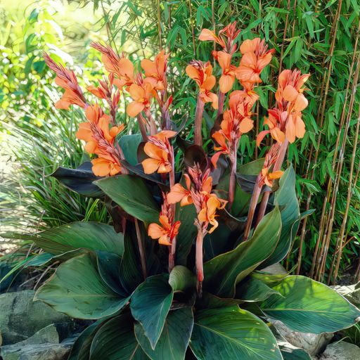
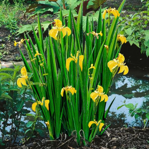
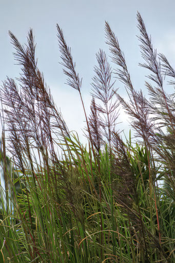
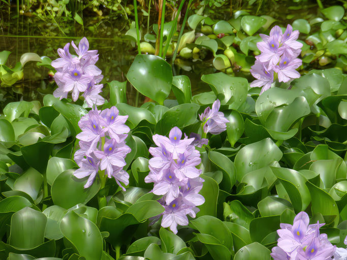
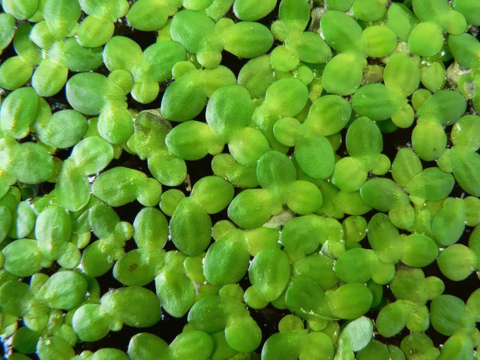
Polyculture: The AquaSai Principle
AquaSai systems always use polyculture — deliberately mixing 3–8 species per cell. Research and field observation confirm that polycultures consistently outperform monocultures:
🔬 Deeper Redox Zonation
Different root architectures (deep tap roots, shallow lateral mats) create more complex redox gradients than any monoculture.
🛡️ Resilience & Redundancy
Disease, pest pressure, or temperature extremes rarely impact all species simultaneously. Functional continuity is maintained.
🌸 Ecosystem Services
Diverse canopies provide wildlife habitat, aesthetic value, educational potential — integral to AquaSai's co-benefit model.
🌡️ Seasonal Complementarity
Different species peak in summer vs. winter, maintaining year-round treatment performance even in temperate climates.
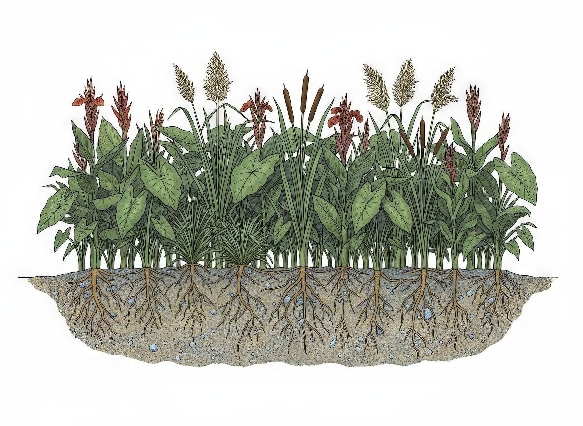
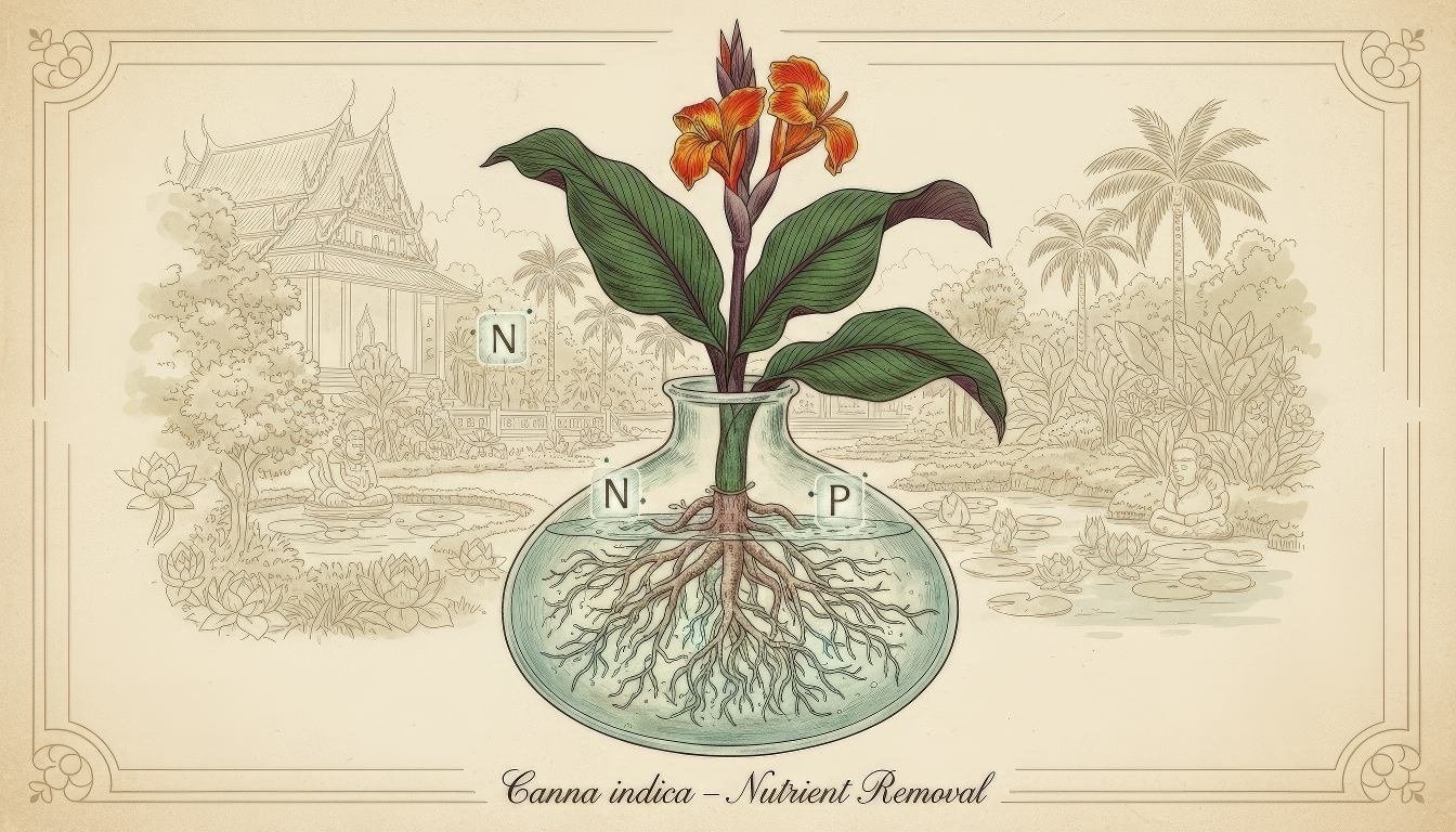
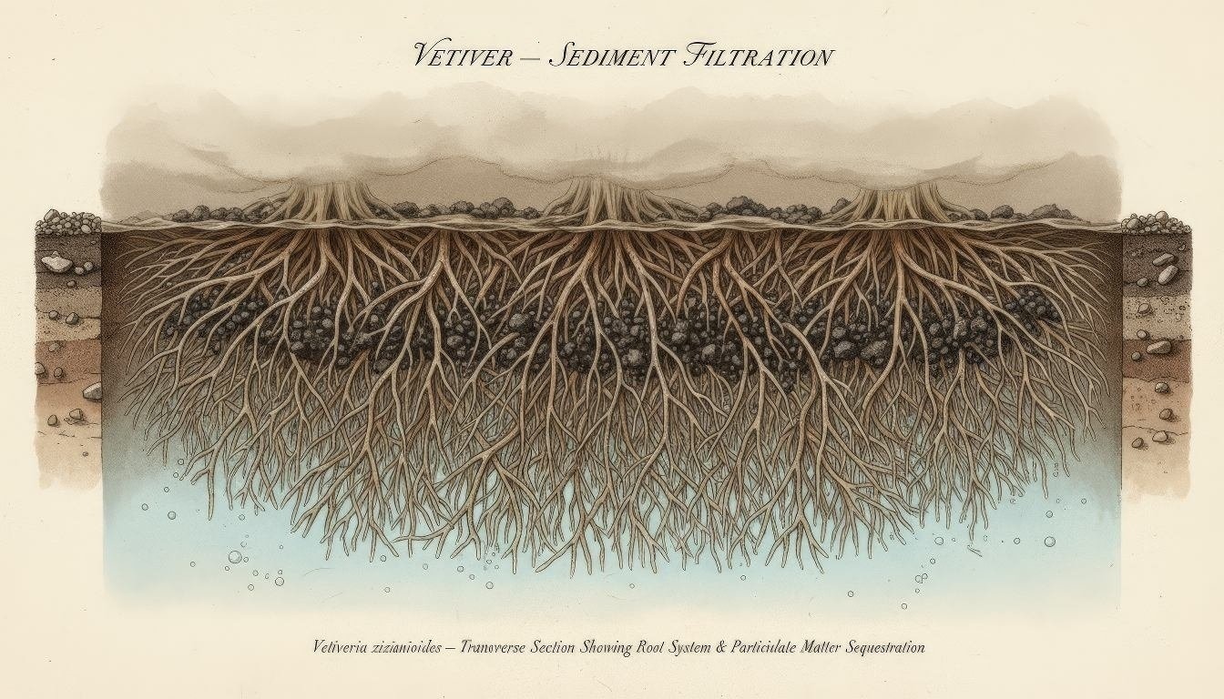
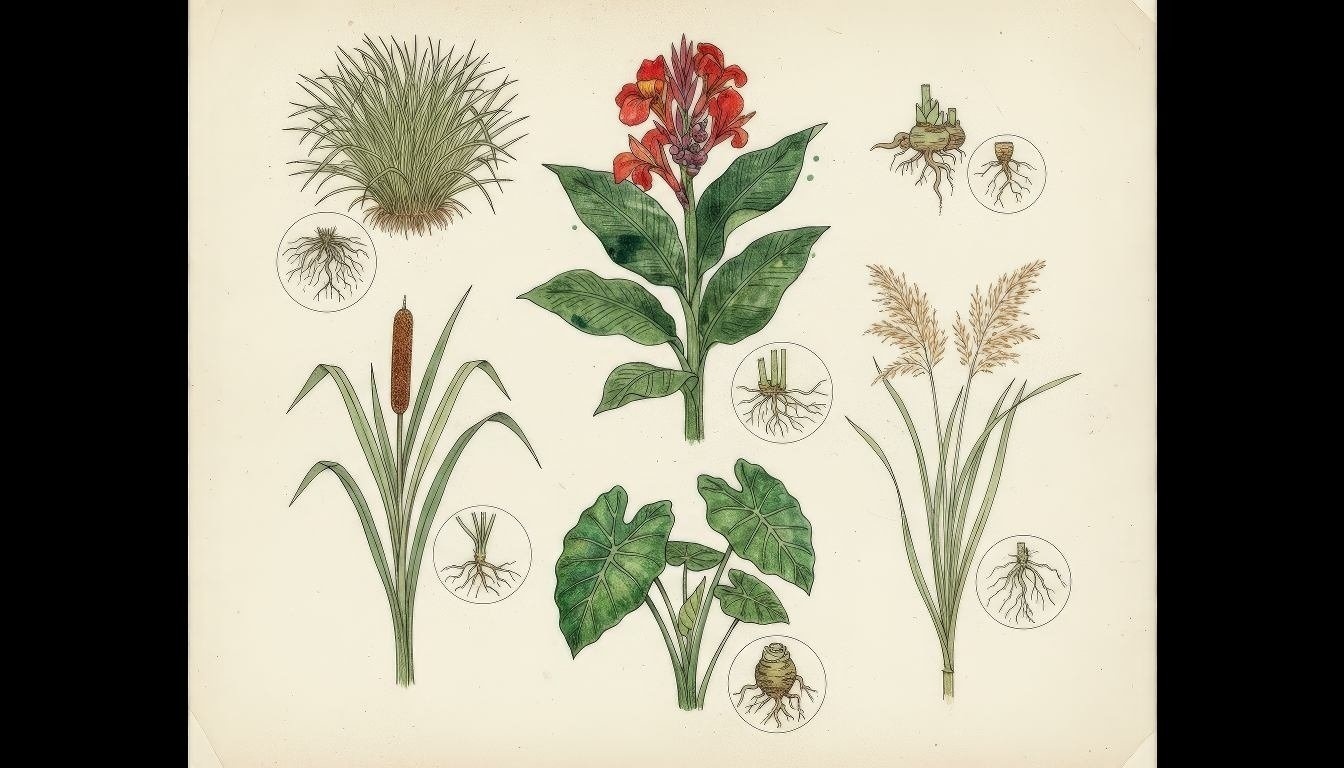
Vetiver (Chrysopogon zizanioides) roots can reach 3–4 m deep in a single season — anchoring banks, mining nutrients and creating vast biofilm surface. AquaSai pairs it with canna, iris and reeds so root depths and bloom seasons complement rather than compete.
The polyculture plates shown here mirror the planting architecture AquaSai used in Nepal — a layered assemblage that keeps the bed productive across the year and doubles as a botanical amenity rather than an eyesore.
— AquaSai plant-ecology library📝 Module 4 Quiz
- Plant selection should balance treatment function, climate resilience and local biodiversity
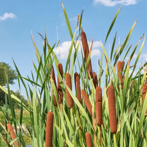
- Phragmites australis dominates globally but native alternatives (Typha, Juncus) offer ecological co-benefits
- Root oxygen release (ROL) from VSSF plants creates aerobic micro-zones critical for nitrification
- Macrophyte biomass and litter decomposition are significant internal nutrient cycles — harvest may be needed